Optimizing streaming ASR on Arm®︎ edge devices with ExecuTorch

This post was co-authored by Josiah Davis, Principal AI Engineer at Arm, and Kshitij Sisodia, Principal Software Engineer at Arm.

---

When you are speaking to a device, you expect text to appear as you talk. That makes streaming automatic speech recognition (ASR) a different challenge from batch transcription, where the model has the complete recording before it starts. Strong batch accuracy does not necessarily carry over into streaming. One cross-model ASR study illustrates this gap. Qwen3-ASR-1.7B achieved the best batch accuracy among the models tested, but its word error rate (WER) rose by 77% when evaluated with 2.4-second audio chunks. 

In that study’s cross-model streaming comparison (Table 5), NVIDIA® Nemotron  Speech Streaming 0.6B had the lowest average streaming WER when operating over 560 ms audio chunks. The comparison makes a critical point: accuracy must be measured at the chunk cadence used in deployment. 

This case study takes the newer, multilingual Nemotron 3.5 from PyTorch to ExecuTorch and profiles its on-device execution on a Google Pixel 11. We ask how precision and chunk size change streaming quality, how much processing time the audio requires with one inference thread, where the workload spends its time, and which native kernels run. The goal is a practical way to evaluate accuracy and latency together. 

In this blog post, you will learn: 

1. How ExecuTorch connects PyTorch models to optimized Arm CPU kernels. 
2. Why streaming ASR needs its own quality evaluation, and how longer chunks improve final-transcript accuracy at the cost of higher latency. 
3. How Arm Scalable Matrix Extension 2 (SME2) reduces total ASR processing time with FP16 and INT8 quantization using per-channel weights (QC8W). 
4. How to combine model operator timings and native kernel samples to understand performance and identify remaining bottlenecks. 
5. How to choose chunk size and precision together to meet your accuracy and latency targets. 

From PyTorch model to CPU instructions

ExecuTorch is PyTorch’s edge inference framework, with export tools and a lightweight runtime. The export process prepares the model for inference and produces a .pte file that the device runtime can load and execute.

Supported operations are delegated to XNNPACK, a CPU inference library. On Android , XNNPACK can select microkernels from Arm® KleidiAI software: small, optimized routines that perform the inner matrix calculations. Operators not delegated to XNNPACK run using ExecuTorch’s portable CPU kernels. 

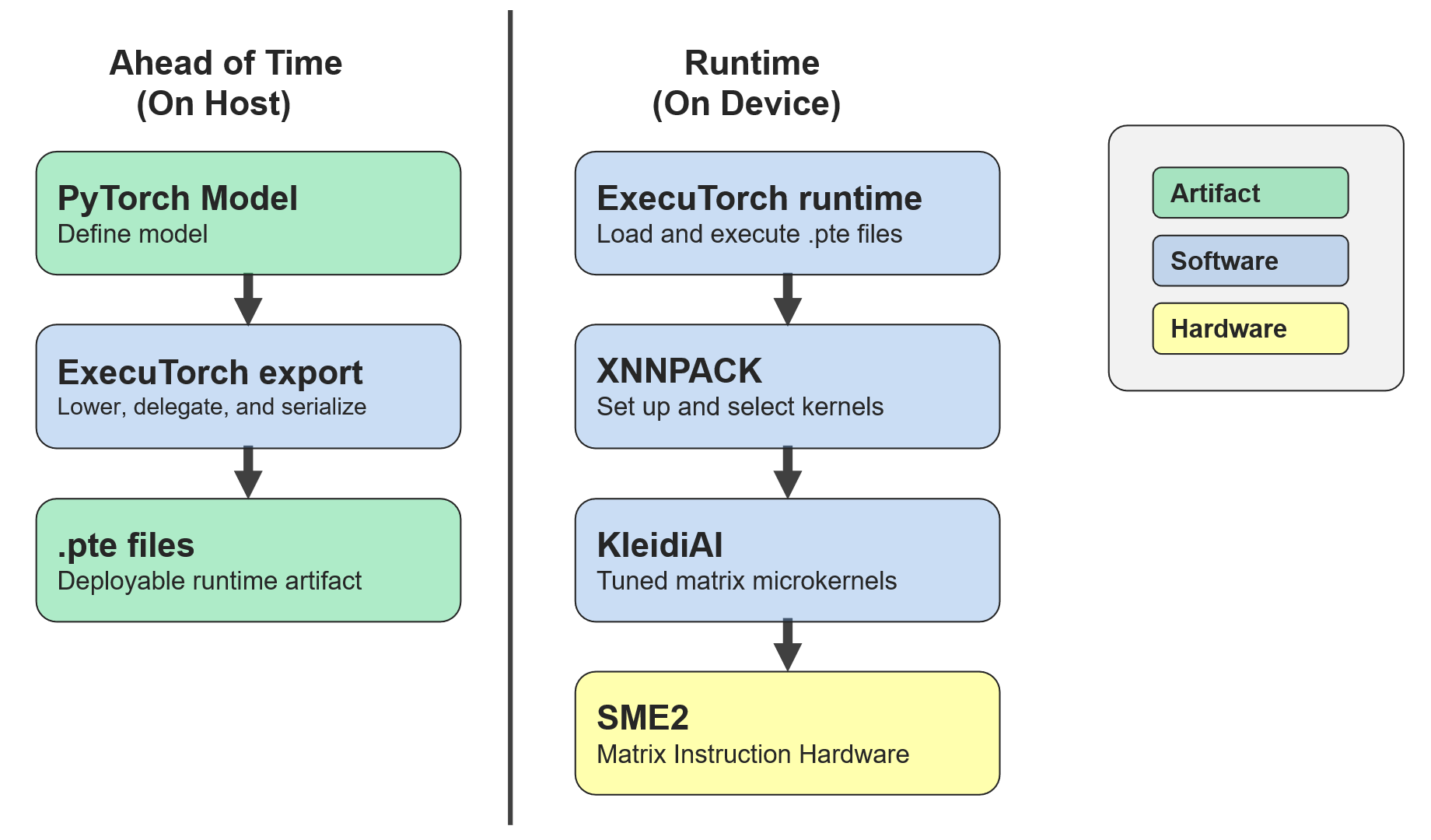
SME2 extends Arm’s instruction set to accelerate matrix calculations, including general matrix multiplication (GEMM). In the Arm C1 CPU cluster implementation with SME2, the matrix unit is shared by cores in the CPU cluster, and KleidiAI provides microkernels that use it for supported operations. Enabling SME2 in a build makes those paths available. However, native profiling is needed to show which kernels actually ran. 

What one streaming call contains

Nemotron 3.5 is a multilingual streaming ASR model built around an RNN-T architecture with three parts: 

1. The encoder uses FastConformer attention and convolution layers to represent the audio. 
2. The predictor uses an LSTM to represent the history of emitted tokens. 
3. The joiner uses a small feedforward layer to combine the encoder’s audio representation with the predictor’s token-history representation and predict the next token. It can also produce a blank, which advances decoding to the next audio position. 

The frontend converts audio into log-mel feature vectors, producing one vector for every 10 ms. The encoder reduces the number of time positions by a factor of 8, so its output has one position for every 80 ms of audio. This creates a more compact sequence representing the same audio duration. 

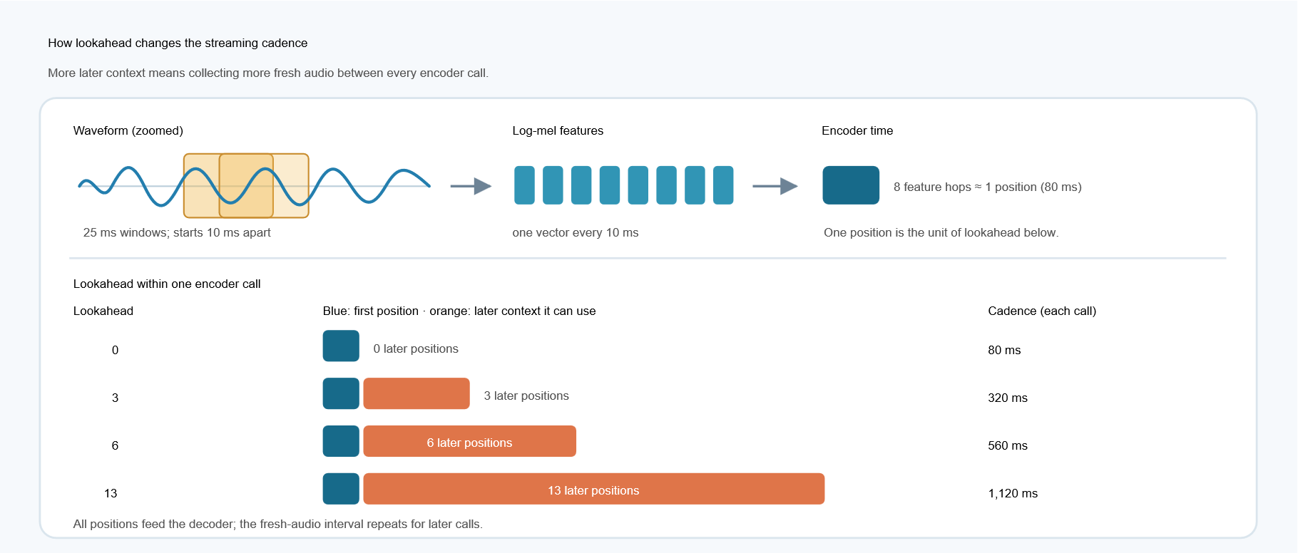
Lookahead is the future context available within a chunk; chunk cadence is how often fresh audio is collected for a call. At lookahead 13, a call collects 1,120 ms of audio and produces 14 encoder positions. The predictor and joiner processes all 14 valid positions, accumulating their tokens into the transcript. 

Lookaheads 0, 3, and 6 give 80, 320, and 560 ms chunks. Longer chunks increase the wait for the first text and subsequent updates; preprocessing and inference add time after audio collection. 

Choose chunk size and precision together

We measured transcription accuracy on the host using the ExecuTorch runtime with its XNNPACK CPU backend. We created a local streaming adapter that uses the Hugging Face Open ASR Leaderboard evaluation harness for dataset preparation, transcript normalization, and WER scoring. 

We evaluated FP32, FP16, and INT8 at four chunk sizes. The INT8 specification is QC8W which uses dynamic INT8 activations and per-channel INT8 weights for eligible linear operations, with FP32 outputs. 

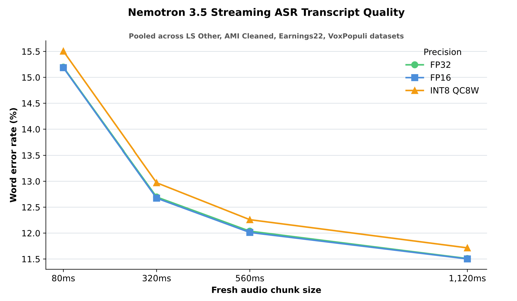
Each point on the above figure covers 14,019 utterances from LibriSpeech Other (LS Other), AMI Cleaned, Earnings22, and VoxPopuli Cleaned AA datasets. WER divides total word errors by total reference words across all four corpora. 

Longer chunks improve final-transcript accuracy. From 80 to 1,120 ms, FP16 WER falls from 15.2% to 11.5%, and QC8W from 15.5% to 11.7%. FP16 essentially matches FP32, differing by less than 0.03 percentage points at every chunk size, so we exclude FP32 from further performance analysis. QC8W preserves strong accuracy, adding 0.21–0.31 percentage points of WER relative to FP32. 

These host WER results inform precision and lookahead choices. However, it does not measure how long it takes for text to appear on the device. 

Test the real-time budget on an edge device

We processed a 24.9-second recording on a Google Pixel 11 smartphone device using 1,120 ms chunks and one inference thread pinned to a mid-core CPU. We chose the mid-core CPU as a representative target for a sustained streaming workload on the system. We tested two builds of ExecuTorch 1.3.1, toggling SME2 support on and off. Each build retained XNNPACK and KleidiAI, and used identical model artifacts. 

Each configuration had two warm-ups and one measured tracing run. Totals cover processing the loaded recording from audio preprocessing through final detokenization. 

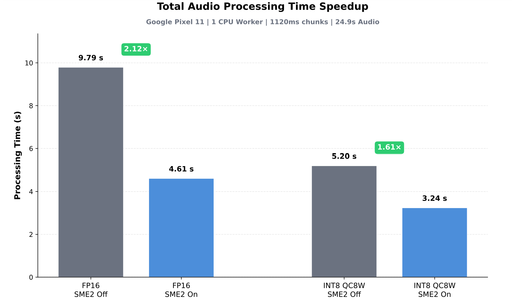
SME2 substantially reduces processing time: FP16 falls from 9.79 to 4.61 seconds (2.12x faster), and QC8W from 5.20 to 3.24 seconds (1.61x faster). 

With and without SME2, both process the recording in much less time than its audio duration. Dividing the processing time by the audio duration we calculate real-time factors of 0.19 for FP16 and 0.13 for QC8W (with SME2 on). This provides substantial processing headroom with only a single inference thread. Audio still has to arrive before it can be decoded, so this headroom does not remove the chunk-collection delay. But it leaves capacity for other CPU work between chunks and can help manage thermal load during sustained transcription. 

Find the bottleneck with ETDump

ETDump records ExecuTorch operator events and timings. To understand where the 2.12X FP16 and 1.61X QC8W speedups come from, we grouped machine learning (ML) operators across the encoder, predictor, and joiner into categories: 

• GEMM (blue): Matrix multiplication, mainly the encoder’s dense layers. 
• Data movement (orange): Copies, concatenation, repeats, and embedding lookup. 
• Elementwise (red): Activations, comparisons, and other per-value work. 
• Convolution and normalization (green and purple): Convolution filters and normalization operators; both are relatively small here. 
• Other (violet): Small remaining timed operations, such as tensor creation. 
• Overhead (gray): Full-run time outside the grouped operator events; this can include runner and framework overhead.

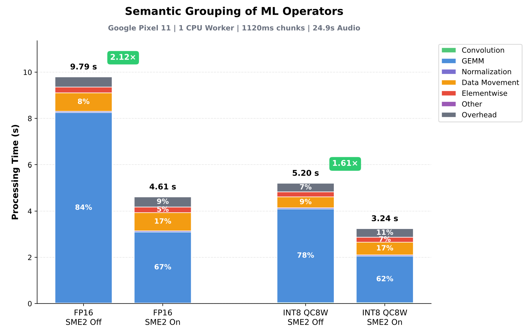
ETDump times are summed across the encoder, predictor, and joiner networks. Adding residual overhead gives the full processing time shown in Figure 4. 

GEMM drives most of the speedup. 

Enabling SME2 reduces GEMM time from 8.2 to 3.1 seconds for FP16 and 4.1 to 2.0 seconds for QC8W. GEMM remains the largest part of the run, though its share of total processing time falls from 84% to 67% for FP16 and 78% to 62% QC8W. Data movement takes roughly the same time for both builds, so its relative share grows as GEMM accelerates: from 8% to 17% for FP16 and 9% to 17% for QC8W. This remaining work limits the overall speedup and offers a target for further optimization. 

Which kernels ran?

ETDump locates the expensive operator families, but does not name the native microkernels that execute them. 

Arm Streamline allows us to sample native call paths and measure hardware counters. On the Pixel 11, we measured 38.4% SME utilization for FP16 and 53.7% for QC8W. This indicates how much of each capture the matrix hardware was allocated; it is not a percentage of peak arithmetic throughput. We also sampled GEMM functions to identify the microkernels selected by each build. 

The function names reveal the sampled paths. The _sme2_mopa suffix denotes a matrix outer-product accumulation routine. NEON and I8MM are the vector instruction families used by the control paths. 

Precision	SME2	Sampled GEMM paths and functions
FP16	True	KleidiAI FP16 SME2  kai_kernel_matmul_clamp_f16_f16p2vlx2_f16p2vlx2_2vlx2vl_sme2_mopa    XNNPACK FP16 NEON  xnn_f16_gemm_minmax_ukernel_6x16__asm_aarch64_neonfp16arith_cortex_a75
FP16	False	XNNPACK FP16 NEON  xnn_f16_gemm_minmax_ukernel_6x16__asm_aarch64_neonfp16arith_cortex_a75
QC8W	True	KleidiAI INT8 SME2, FP32 output  kai_kernel_matmul_clamp_f32_qai8dxp1vlx4_qsi8cxp4vlx4_1vlx4vl_sme2_mopa    KleidiAI FP32 SME2  kai_kernel_matmul_clamp_f32_f32p2vlx1_f32p2vlx1biasf32_sme2_mopa
QC8W	False	KleidiAI INT8 NEON I8MM, FP32 output  kai_run_matmul_clamp_f32_qai8dxp4x8_qsi8cxp4x8_16x4_neon_i8mm

These captures confirm that SME2-targeted KleidiAI GEMM kernels ran on the Pixel 11 for both FP16 and QC8W, alongside other kernel paths. In the FP16 build, some GEMM operations still use NEON. In the QC8W build, some GEMM operations still run in FP32. 

This highlights a tooling gap in the ecosystem. ETDump exposes model operator timings, while Streamline samples native functions, but neither tool directly connects these views. Mapping individual model layers to the observed kernel functions remains future work. 

Choosing an operating point

Deployment involves balancing response latency and accuracy across precision and chunk size. An application might start with an accuracy target or a latency budget; the following examples illustrate both approaches. 

Figure 6 below pairs the host WER results with a Pixel 11 component benchmark for SME2-enabled FP16 and QC8W. Grey ticks mark when audio collection finishes; dotted segments add the measured compute delay. 

The x-axis is a conditional time to first-token estimate: audio collection time plus the median encoder–predictor–joiner sequence time. The component benchmark used synthetic input, fresh stream state, and 75 measured samples per configuration across three rounds. It assumes that the first output emits text. 

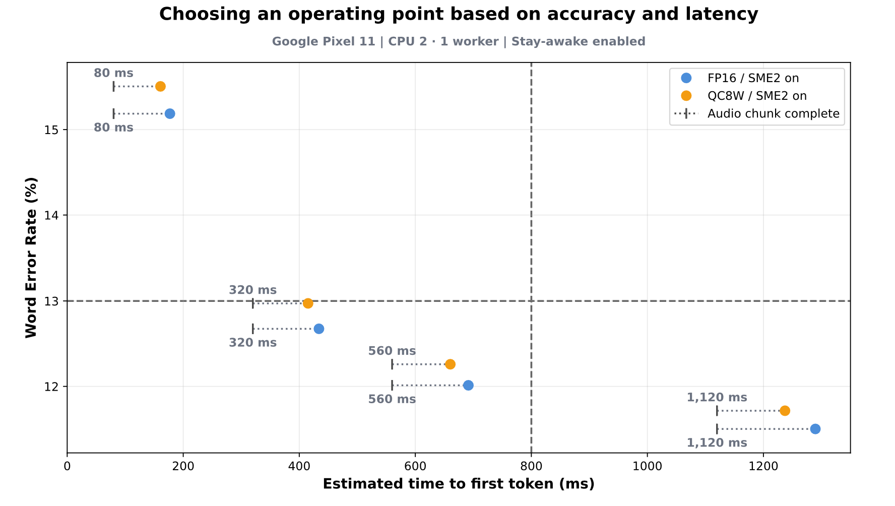
For an illustrative 13% WER ceiling, both FP16 and QC8W qualify at 320, 560, and 1,120 ms chunk sizes. The 320 ms chunks favor earlier responses, with 12.67% WER for FP16 and 12.97% for QC8W. Longer chunks improve accuracy, reaching 11.50% and 11.72%, respectively, at 1,120 ms, but require more audio to arrive before transcripts begin to appear. 

For an 800 ms latency budget, both precisions at 320 ms and 560 ms fall within the budget and also below the illustrated 13% WER ceiling. The 320 ms configurations favor earlier responses while 560 ms gives better accuracy. At 560 ms, FP16 combines 12.01% WER with an estimated 691 ms delay, while QC8W combines 12.26% with 660 ms. Here, both 80 ms configurations miss the WER target. Conversely, both 1,120 ms configurations miss the latency budget.

What this means for developers 

• Evaluate streaming ASR at the intended chunk size. Whole-recording accuracy does not predict streaming quality. Longer chunks improve final-transcript accuracy here, while increasing response latency. 
• ExecuTorch connects PyTorch models to optimized Arm CPU kernels. Its export and runtime path lets XNNPACK select KleidiAI microkernels for eligible operations. 
• SME2 creates more processing headroom. Accelerating matrix work reduces the time spent on ASR, leaving more room for other application tasks or concurrent workloads on the device. 
• ETDump reveals operator speedups and remaining bottlenecks. Grouping operator timings shows where the gains come from and how data movement becomes a larger share of processing time. 
• Streamline identifies the native microkernels that ran. Native samples confirm selection of SME2 kernels, while hardware counters show matrix hardware allocation. 
• Choose chunk size and precision together. Comparing precision and chunk-size combinations helps developers balance response latency against transcript accuracy for their application.